Continuous Futures — Construction Methods

Before we will carry out a certain methodology, we will visit some common procedures to generate a continuous time-series. For all this, there is some terminology needed, which frequently comes with Futures. For our purposes we will refer to front and back contracts, where the front contract is the first Futures due for expiry, while the back contract matures later by a particular frequency (often one or three months after the front contract). In the context of comparing the prices between two subsequent Futures, a higher price in the back contract is referred to as contango, while we speak of backwardation in case of the opposite price relationship. Another important aspect is the tick size and the tick value of a contract. Tick size refers to the smallest possible price movement and tick value is the loss or gain incurred by that movement.

So first of all, we have to ask, why there is a difference in the price in subsequent Futures contracts at all? To gain an understanding of this, one way is to follow the close link between Futures contract and underlying, and at the same time acknowledge that, — given an arbitrage free world — a holding, whether in the underlying or the Futures, will yield exactly in the same payoffs for the investor. So more precisely, the cost of holding the underlying until the next respective expiration date, determines the gap between two contracts. Depending on the market, those influence factors can be repo rates, dividends, storage costs, etc.

Before we start implementing algorithms to come up with a Continuous Futures time-series, we will shortly discuss the most prominent techniques available in that space.

1. Splicing contracts together with no adjustments

This is the typically done already by market data providers like Bloomberg or Reuters (FGBLc1 for the spliced Bund for instance). We will (possibly) end up in a price jump on the day when contracts are switched. In case trading signals (see second article) are extracted from those series, we rely on a mix of inputs from both contracts potentially yielding a biased result as the price jump is inherited in the calculations. We also receive a distorted picture with regards to backtesting the PnL of any strategy relying on such a time series. Just imagine a MACD strategy would make you buy just before the front contract matures and sell straight after in the back contract (or the then front contract at the point in time of selling). Assuming a contango you would clearly overstate your profit.

2. Splicing contracts together with explicitly accounting for a roll over

In the above mentioned MACD strategy example, we would clearly correct the inflated PnL by selling the front contract and buying into the back contract simultaneously at or just before expiry. Afterwards, we would then sell the former back contract (being the new front contract by now) correctly reflecting the price jump in our performance measurement. But still, we are left with biased signals from strategies relying on both contracts.

3. Continuously adjusting the contracts over time ("Perpetual Method")

In a nutshell, the Perpetual Method applies weights to front and back contract over a pre-defined period of time. So to say, we trade out of the "old" contract into the "new" in a linear fashion. For instance, if we assume 5 roll over days, we do the weighting according to the following scheme:

Applying this method clearly improves the sudden price change introduced by switching to a new contract by smoothing the roll over according to the weighting scheme. Note that trading has also to be set up accordingly to make everything consistent.

4. Splicing contracts together with forward or backward adjustments ("Panama Adjustment")

The Panama Adjustment either adjusts the actual (forward) or the historical (backward) contracts, such that they align in a smooth fashion on expiry date. While overcoming the distortion on signal generation due to a smooth time series, we are left with biased relative price performance stemming from absolute series adjustments (the absolute gaps between contracts). This can also leads to potentially strong data trends, especially over long time horizons (with even the possibility of negative prices). However, the prior PnL or performance unit of Futures is the tick value, which still can be easily interpreted correctly, even if we would analyze a time series trending away substantially from the original Futures prices.

As mentioned above, we we pick German Government Bond Futures (Schatz, Bobl, Bund) for our analysis. We collect daily OHLCV ("Open", "High", "Low", "Close", "Volume") market data for the respective securities in a dict of Pandas DataFrames. Thomson Reuters Eikon offers Continuous ("spliced together") Futures data by calling the ticker symbol (i. e. "FGBL" for the Bund) and "c1" and "c2" for the continuous front and back contract. The following code will do this for us:

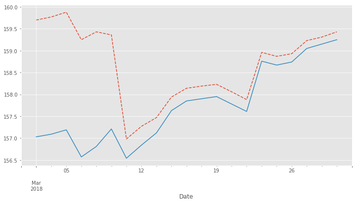
We can easily visualize the roll gap for the Bund March '18 roll with Matplotlib. Below you see the front contract ("FGBLc1", dashed red line) and the back contract ("FGBLc2", blue solid line). On the 8th, "FGBLc1" expires and therefore "FGBLc2" becomes the new "FGBLc1". That is why you see the sudden drop in the time-series.

To implement the Perpetual Method as outlined above, we define a function "get_perp_fut". The function basically takes the already fetched DataFrames consisting of spliced front and back contracts as "market_data" argument. Additionally, the rollover days and the data columns can be specified. Below is the Python representation of that function:

Probably the best way of seeing how our just created Continuous Futures performs is to visualize the outcome. Again we use Matplotlib and specify 10 and 40 days respectively as rollover period. We also include our Spliced Contracts series as benchmark.

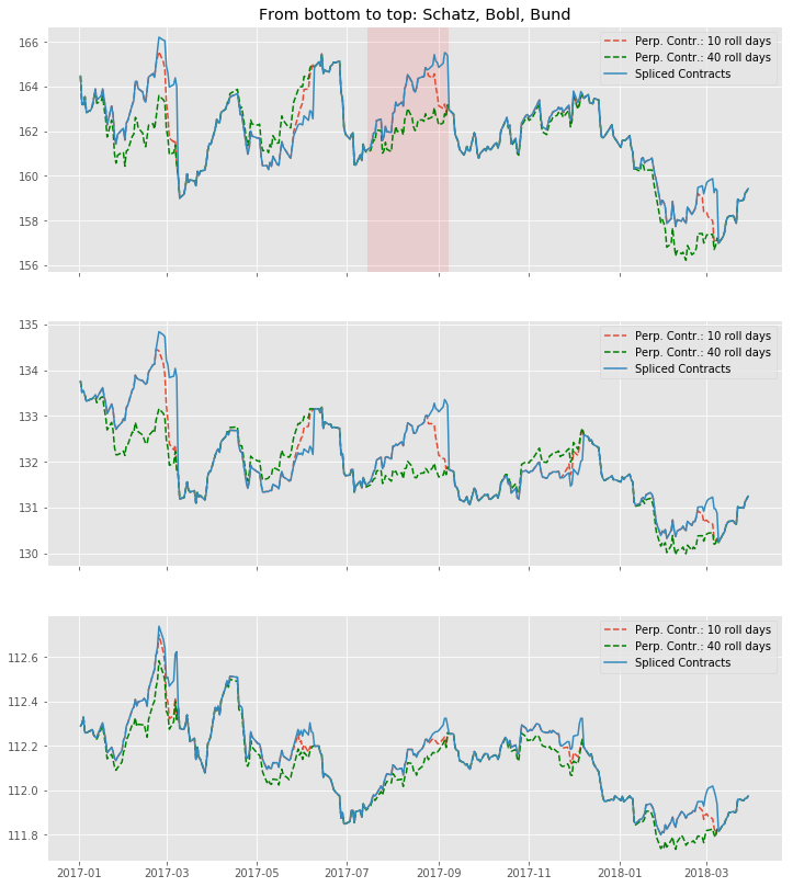
We can conclude that — given the large roll gaps especially for Bobl and Bund — , a longer roll period enhances the "smoothness" of the time-series. But still, even if we use 40 days, we amend our data in a way that is probably not a perfect fit. For instance, consider the highlighted area in the Bund chart: For 10 roll days we completely miss the daily market directions. On those 10 days, we are dragged down by the roll gap, such that we artificially create a downward trend that never really existed. If we look at the 40 roll days, we are clearly able to better capture the daily movements, but still, we are missing another element, which is the slight upward trend during the roll. To make the Perpetual Method a better fit, we would even have to lengthen the rollover further. By this we would run into other areas of trouble, namely an illiquid back contract and a hugely complex trading in case we want to do this consistently to our rollover.

Here we proceed basically the same like above: From our simple spliced contracts we form a smooth time series by defining a Python function doing the heavy-lifting for us. To be in line with prices in the market, we keep the most recent data unadjusted and cumulate the roll gap backwards over time. As the basis of the relevant Futures prices tend to be quite volatile just before the roll, we average the 4 trading days just before expiry. Given an absence of a particular view on price direction during roll, that makes sense to limit risks in trading, if the actual position is rolled over accordingly (we borrow a bit from the Perpetual Method here).

The code snippet below will illustrate our methodology:

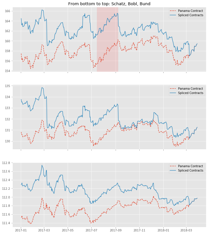
We again visualize the outcome with Matplotlib. The most encouraging point can be seen at a first glance: Even with large roll gaps, we don’t introduce some new, non existent trends into our data. Of course, we pay the price with a growing and growing divergence from the real data if we travel backwards in time. But again, this seems to be a price worth paying, if we interpret our data correctly.

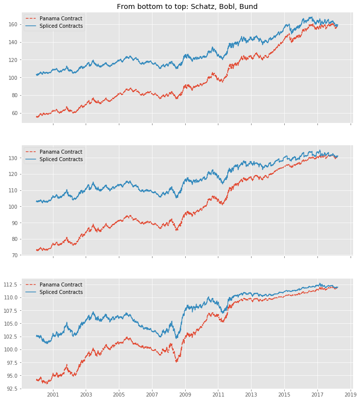
To get a better feeling of how a even longer time-series would be changed, here are our contracts with the Panama Method back as far as 2000-1-1 (a period which was almost entirely a bull market for government bonds). You can see how nice being long over that period would have been, as carry even enhances the stellar return for the buyer.